HRV measurements: duration

Blog post by Marco Altini.

In the last post I covered the importance of context when interpreting HRV data, and pointed out that the optimal routine involves a morning HRV measurement, since this is the easiest way to isolate context and limit the impact of other stressors.

Other important aspects, beyond when to take the measurement, are the measurement duration, type (lying, standing or orthostatic), paced breathing, and frequency (how often?). In this post, I will cover measurement duration. In particular, I will reference to a recent study by Michael Esco and Andrew Flatt, and try to replicate and extend some of their work. 

Esco and Flatt (see the full paper here) were interested in determining if a $60$ seconds measurement is sufficient for valid assessment of HRV, in particular of $ln(rMSSD)$, a metric often used as a proxy to parasympathetic activity when monitoring training load. Their reference was the same metric ($ln(rMSSD)$) over a longer (standard) window of $5$ minutes. In their study population ($23$ collegiate athletes), $60$ seconds seemed sufficient to obtain HRV measures as good as the reference, while shorter measurements were a bit more problematic, especially the $10$ seconds one. However, no statistically significant difference was found between any time window.   

In my analysis I will look at windows of $10$ s, $30$ s, $60$ s and $5$ minutes, as done by Esco and Flatt, as well as for $3$ minutes recordings, since HRV4Trainings provides a choice between $60$ s, $3$ minutes and $5$ minutes, and in general, the shorter the more practical. For this analysis I will also look at rMSSD and not only $ln(rMSSD)$. 

Dataset

For this analysis I used a dataset I collected for another study I designed during my PhD. More details can be found here. Long story short, in my research I was measuring energy expenditure, and therefore I also recorded most of the data in the morning in laboratory settings. Participants were required to restrain from drinking (except for water), eating and smoking in the 2 hours preceding the experiment, similarly to what was required by Esco and Flatt. Data was collected using the ECG Necklace, a device that measures ECG and acceleration.

My participants were however mainly university employees or students, and therefore less fit than the collegiate athletes of the original study. For my protocol, participants went through a series of physical activities (lying, sedentary, household, walking at different speeds, running, biking - $VO_2$max test). Here I isolated the first 20 minutes of data for each participant and highlighted the "lying" part in the RR intervals time series, which I detected using accelerometer data (since the sensor is on the chest, this step is rather easy):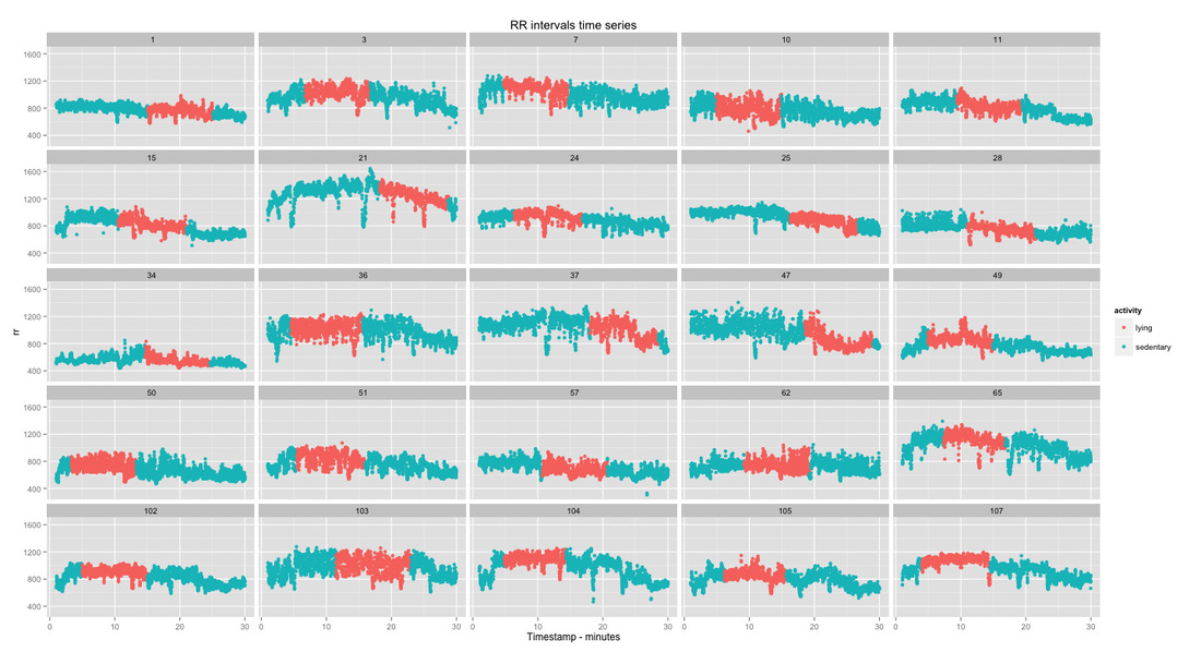

The only preprocessing here was the removal of consecutive RR intervals differing more than $20\%$ and discarding participants where the overall noise was more than $1\%$ of the data. This step was to avoid HRV features to be affected by ectopic beats or other motion artifacts or noise in general. I ended up with $25$ participants.

Analysis of different time windows

As a next step I computed time and frequency domain HRV features over the RR intervals marked as "lying", so discarding all the remaining data. This is typically a $10$-$15$ minutes segment (see data highlighted in red above). Features are computed over windows of $10$ seconds to $5$ minutes (non-overlapping). Therefore we will end up with many $10$ s windows and just a few $5$ minutes windows (our reference). If I understood it correctly, in the original paper Esco and Flatt randomly picked one of these time window as a comparison. Here I decided to keep all of them so that I could look at their distribution. For the Bland-Altman plots, I computed the mean of the values over a certain window length and participant, and used that value as the comparison one, instead of selecting one randomly.

Let's look at rMSSD for different time windows and participants. Each color is a participant, and for each participant we see boxplots for the different conditions (i.e. time windows). By looking at boxplots we can easily see how the values are distributed and visually compare across time windows. Time windows are ordered by length, from $10$ s to $5$ minutes: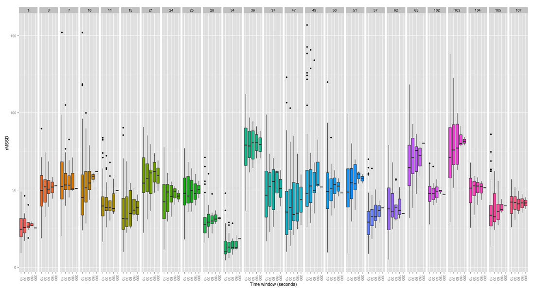

What can we derive from the plot above?

In general, we can see positive results, with rMSSD values being quite stable over different time windows. For each participant, the median of the boxplot (black line) doesn't differ much across different time windows. However, the variability (spread of the distribution) is quite high for $10$ s windows, while it seems to get already much better for $30$ s. It is important to note that HRV is never constant and even the reference measure (i.e. recording over 5 minutes) can change quite a bit over a $10$-$15$ minutes period. We can spot these differences in our $5$ minute reference window for the few participants were "lying" was longer than $10$ minutes, for example participant $107$.

Similarly, plotting $ln(rMSSD)$: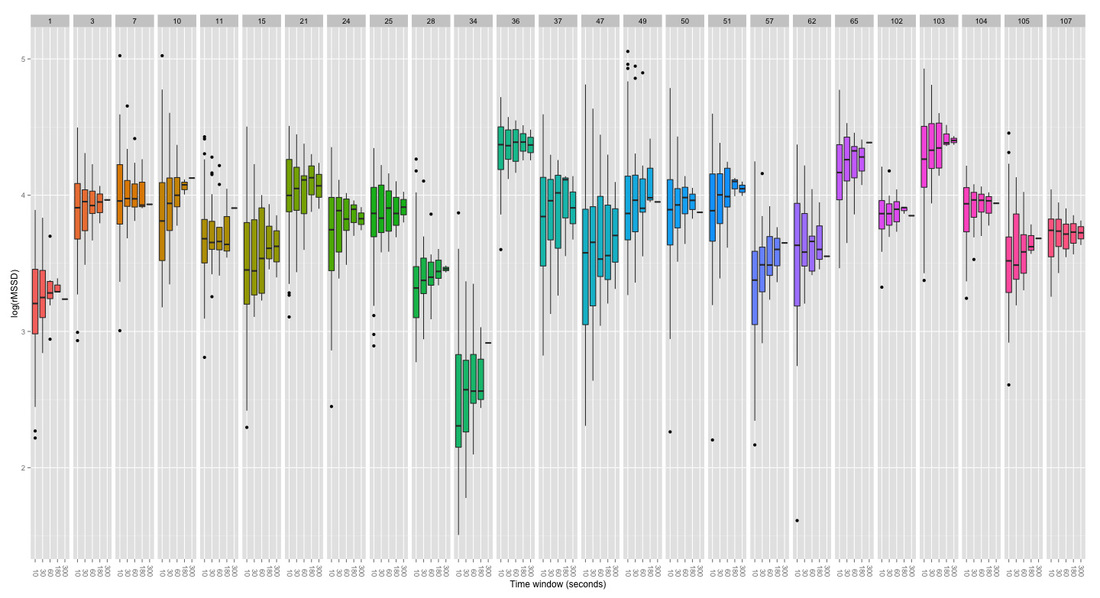

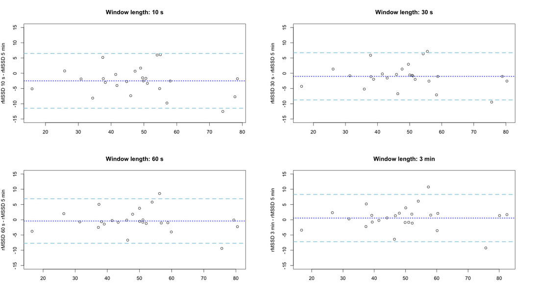
Finally, we can look at bias and limits of agreement using Bland-Altman plots. First rMSSD:

and then the logarithmic version:

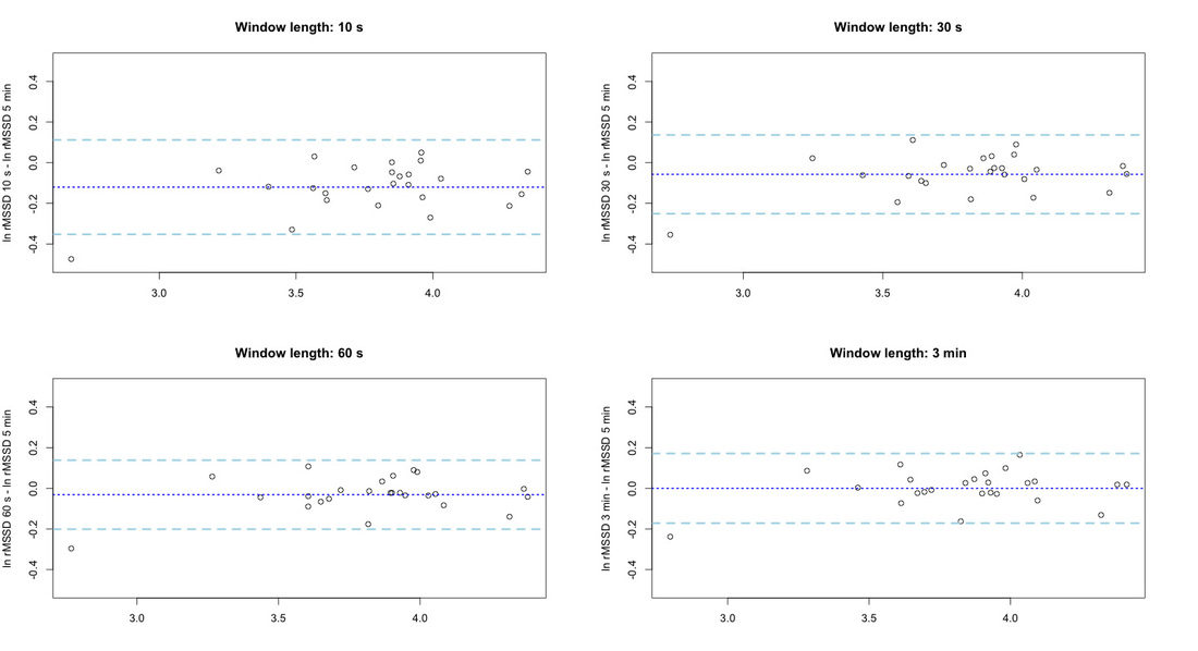
As we could expect, we have reduced bias with increased window length. An analysis of variance (ANOVA) shows no significant differences between conditions (i.e. between time windows), when using the mean over the different windows to represent the HRV value. The same was reported by Esco and Flatt, who also computed the intra-class correlation (ICC), and showed a decrease in ICC as the window size decreased. From the spread that we can see in the previous boxplots, I would also suggest longer windows to be preferable.

Summary

The dataset used for this analysis was not collected with the intention of measuring HRV and the protocol was not exactly the same as the one of the original study by Esco and Flatt, however, I could replicate fairly well their findings. $60$ seconds seem to be a sufficient time window for morning HRV measurements even though, according to my data, the best results are shown when we use a $3$ minutes window. 

While $60$ seconds showed limited spread and good agreement with the reference $5$ minutes, shorter measurements are probably not a good idea. No statistically significant differences were found in either the study by Esco and Flatt and my analysis, however, $10$ seconds is a very short window even for a rather stable measure such as rMSSD. Especially at rest conditions and in trained participants, $10$ seconds could be as short as one single breathing cycle.

Clearly, there are many trade-offs to consider. Especially when using the camera version of HRV4Training, I strongly advise to use the short $60$ seconds time window, since performing the PPG measurement for more than $60$ seconds will increase the risk of moving the finger, and therefore affecting negatively the measurement due to motion artifacts.

Follow @marco_alt